Introduction
Overview
Teaching: 10 min
Exercises: 5 minQuestions
What parallel computing is and why it is important?
How does a parallel program work?
Objectives
Explain differences between a serial and a parallel program
Introduce types of parallelism available in modern computers
Why to learn parallel computing?
-
Building faster serial computers became constrained due to both physical and practical reasons.
-
The increase in serial performance slowed down because processor designs approached limits of miniaturization, clock frequency, power consumption, data transmission speed.
-
It is increasingly expensive to make a single processor faster. Using a larger number of moderately fast commodity processors to achieve the same (or better) performance is more practical.
Parallel Computing Applications
Here are just a few examples of how parallel computing is helping to accelerate research and solve the previously unsolvable problems.
- Numeric Weather prediction
- Taking current observations uses mathematical models to forecast the future state of the weather
- Computational Astrophysics
- Numerical relativity, magnetohydrodynamics, stellar and galactic magnetohydrodynamics
- Seismic Data Processing
- Analyze seismic data to find oil and gas-bearing layers
- Commercial world
- Nearly every major aspect of today’s banking, from credit scoring to risk modelling to fraud detection, is GPU-accelerated.
- Pharmaceutical design
- Uses parallel computing for running simulations of molecular dynamics
- Computational fluid dynamics, tidal wave simulations
Benefits of Parallel Computing:
- It allows us to solve problems in a shorter time.
- Allows solving larger, more detailed problems compared to serial execution.
- Overall parallel computing is much better suited for modelling, simulating and understanding complex, real-world phenomena.
Limitations and Disadvantages:
- Some problems can not be broken into pieces of work that can be done independently
- Not every problem can be solved in less time with multiple compute resources than with a single computing resource. Some problems may not have enough inherent parallelism to exploit.
- Could be more costly in equipment (expensive interconnect)
- Coding expertise
- Require time and effort
Before you start your parallel computing project
- Select the most appropriate parallelization options for your problem.
- Estimate the effort and potential benefits.
In this lesson, we hope to give you knowledge and skills to make the right decisions on parallel computing projects.
How does a Parallel Program Work?
Parallelism is the future of computing. Parallel programming allows us to increase the amount of processing power in a system. How does a parallel program work?
Traditional serial program

- A problem is broken into a set of instructions
- Instructions are executed sequentially on a single CPU
- Only one instruction can be executed at a time
Parallel program
- Parallel computing is breaking a problem into smaller chunks and executing them concurrently on a set of different CPUs and/or computers.

- A problem is broken into parts that can be done concurrently
- Each part is further broken down into a set of instructions
- Instructions from each part execute simultaneously on different processors
-
Requires an overall execution control & coordination mechanism.
-
Modern desktop/laptop computers come equipped with multiple central processing units (cores) that can process many sets of instructions simultaneously.
-
Each core is equipped with a vector unit that can process multiple data at one time. Vector units are described by the number of the bits that the vector unit can process at one time. For example, a 256 bit-wide vector unit can process four double-precision floating point numbers simultaneously.
- Networks connect multiple stand-alone computers (nodes) to make larger parallel computer clusters.
For example, a typical Compute Canada cluster has thousands of computers (network nodes):
- Each compute node is a multi-processor parallel computer
- Each processor is equipped with AVX-2 or AVX-512 vector units
- Multiple compute nodes are interconnected with an Infiniband network
- Special purpose nodes (login, storage, scheduling, etc.)
What fraction of the total processing power can a serial program use?
Let’s consider an 8 core CPU with AVX-512 vector unit, commonly found in home desktops.
- What percentage of the theoretical processing capability of this processor can a double-precision serial program without vectorization use?
- What about a serial program with vectorization?
Solution
- 8 cores x (512 bit-wide vector unit)/(64-bit double) = 64-way parallelism. 1 serial path/64 parallel paths = .016 or 1.6%
- Full use of 1 of 8 cores = 25%
TOP 500 publishes current details of the fastest computer systems.
- The fastest supercomputer: IBM Summit
- Summit System Overview
- Performance Development
- In the application area statistics “Not Specified” is by far the largest category - probably means multiple applications.

Key Points
Parallel computing is much better suited for modelling, simulating and understanding complex, real-world phenomena.
Modern computers have several levels of parallelism
Parallel Computers
Overview
Teaching: 10 min
Exercises: 0 minQuestions
How is a typical CPU organized?
What are the four major groups of computer architectures?
Objectives
Explain the various criteria on which classification of parallel computers are based.
Introduce Flynn’s classification.
To make full use of computing resources the programmer needs to have a working knowledge of the parallel programming concepts and tools available for writing parallel applications. To build a basic understanding of how parallel computing works, let’s start with an explanation of the components that comprise computers and their function.
Von Neumann’s Architecture
Von Neumann’s architecture was first published by John von Neumann in 1945. It is based on the stored-program computer concept where computer memory is used to store both program instructions and data. Program instructions tell the computer to do something.

- Central Processing Unit:
- the electronic circuit responsible for executing the instructions of a computer program.
- Memory Unit:
- consists of random access memory (RAM) Unlike a hard drive (secondary memory), this memory is fast and directly accessible by the CPU.
- Arithmetic Logic Unit:
- carries out arithmetic (add, subtract etc) and logic (AND, OR, NOT etc) operations.
- Control unit:
- reads and interprets instructions from the memory unit.
- controls the operation of the ALU, memory and input/output devices, telling them how to respond to the program instructions.
- Registers
- Registers are high-speed storage areas in the CPU. All data must be stored in a register before it can be processed.
- Input/Output Devices:
- The interface to the human operator, e.g. keyboard, mouse, monitor, speakers, printer, etc.
Parallel computers still follow this basic design, just multiplied in units. The basic, fundamental architecture remains the same.
Parallel computers can be classified based on various criteria:
- number of data & instruction streams
- computer hardware structure (tightly or loosely coupled)
- degree of parallelism (the number of binary digits that can be processed within a unit time by a computer system)
Today there is no completely satisfactory classification of the different types of parallel systems. The most popular taxonomy of computer architecture is the Flynn’s classification.
Classifications of parallel computers
- Flynn’s classification: (1966) is based on the multiplicity of instruction streams and the data streams in computer systems.
- Feng’s classification: (1972) is based on serial versus parallel processing (degree of parallelism).
- Handler’s classification: (1977) is determined by the degree of parallelism and pipelining in various subsystem levels.
Flynn’s classification of Parallel Computers
- Flynn’s classification scheme is based on the multiplicity of information streams. Two types of information flow into a processor: instructions and data.
- The instruction stream is defined as the sequence of instructions performed by the processing unit.
- The data stream is defined as the data traffic exchanged between the memory and the processing unit.
In Flynn’s classification, either of the instruction or data streams can be single or multiple. Thus computer architecture can be classified into the following four distinct categories:

SISD
Conventional single-processor von Neumann’s computers are classified as SISD systems.
Examples: Historical supercomputers such as the Control Data Corporation 6600.
SIMD
- The SIMD model of parallel computing consists of two parts: a front-end computer of the usual von Neumann style, and a processor array.
- The processor array is a set of identical synchronized processing elements capable of simultaneously performing the same operation on different data.
- The application program is executed by the front-end in the usual serial way, but issues commands to the processor array to carry out SIMD operations in parallel.
All modern desktop/laptop processors are classified as SIMD systems.
MIMD
- Multiple-instruction multiple-data streams (MIMD) parallel architectures are made of multiple processors and multiple memory modules connected via some interconnection network. They fall into two broad categories: shared memory or message passing.
- Processors exchange information through their central shared memory in shared memory systems, and exchange information through their interconnection network in message-passing systems.
MIMD shared memory system
- A shared memory system typically accomplishes inter-processor coordination through a global memory shared by all processors.
- Because access to shared memory is balanced, these systems are also called SMP (symmetric multiprocessor) systems
MIMD message passing system
- A message-passing system (also referred to as distributed memory) typically combines the local memory and processor at each node of the interconnection network.
- There is no global memory, so it is necessary to move data from one local memory to another employing message-passing.
- This is typically done by a Send/Receive pair of commands, which must be written into the application software by a programmer.
MISD
- In the MISD category, the same stream of data flows through a linear array of processors executing different instruction streams.
- In practice, there is no viable MISD machine
Key Points
Parallel computers follow basic von Neumann’s CPU design.
Parallel computers can be divided into 4 groups based on the number of instruction and data streams.
Memory Organisations of Parallel Computers
Overview
Teaching: 10 min
Exercises: 0 minQuestions
How is computer memory in parallel computers organized?
Objectives
Introduce types of memory organization in parallel computers
Discuss implications of computer memory organization for parallel programming
The organization of the memory system is second, equally important, aspect of high-performance computing. If the memory cannot keep up and provide instructions and data at a sufficient rate there will be no improvement in performance.
Processors are typically able to execute instructions much faster than to read/write data from the main memory. Matching memory response to processor speed is very important for efficient parallel scaling. Solutions to the memory access problem have led to the development of two parallel memory architectures: shared memory and distributed memory.
The distinction between shared memory and distributed memory is an important one for programmers because it determines how different parts of a parallel program will communicate.
This section introduces techniques used to connect processors to memories in high-performance computers and how these techniques affect programmers.
Shared memory
- Multiple processors can operate independently but share the same memory resources.
- All processors have equal access to data and instructions in this memory
- Changes in a memory done by one processor are visible to all other processors.
Based upon memory access times shared memory computers can be divided into two categories:
- Uniform Memory Access (UMA)
- Non-Uniform Memory Access (NUMA)

- All processors share memory uniformly, i.e. access time to a memory location is independent on which of the processors.

- Used in multiprocessor systems.
- When many CPUs are trying to access the same memory they can be “starved” of data because only one processor can access the computer’s memory at a time.
- NUMA attempts to address this problem by providing separate memory for each processor.
- CPUs are physically linked using a fast interconnect.
- A CPU can access its local memory faster than non-local memory (memory local to another processor or memory shared between processors).
In a shared memory system it is only necessary to build a data structure in memory and pass references to the data structure to parallel subroutines. For example, a matrix multiplication routine that breaks matrices into a set of blocks only needs to pass the indices of each block to the parallel subroutines.
Advantages
- User-friendly programming.
- Fash data sharing due to a close connection between CPUs and memory
Disadvantages
- Not highly scalable. Adding more CPUs increases traffic on the shared memory-CPU path,
- Lack of data coherence. The change in the memory of one CPU needs to be reflected to the other processors, otherwise, the different processors will be working with incoherent data.
- The programmer is responsible for synchronization.
Distributed memory

- In a distributed memory system each processor has a local memory that is not accessible from any other processor
- Programs on each processor interact with each other using some form of a network interconnect (Ethernet, Infiniband, Quadrics, etc.).
- A distributed memory program must create copies of shared data in each local memory. These copies are created by sending a message containing the data to another processor.
In the matrix multiplication example, the controlling process would have to send messages to other processors. Each message would contain all submatrices required to compute one part of the result. A drawback to this memory organization is that these messages might have to be quite large.
Advantages
- Each processor can use its local memory without interference from other processors.
- There is no inherent limit to the number of processors; the size of the system is constrained only by the network used to connect processors.
Disadvantages
- The complexity of programming: the programmer is responsible for many of the details associated with data communication between processors.
- It may be difficult to map complex data structures from global memory, to distributed memory organization.
- Longer memory access times.
Hybrid Distributed-Shared Memory
 Practically all HPC computer systems today employ both shared and distributed memory architectures.
- The shared memory component can be a shared memory machine and/or graphics processing units (GPU).
- The distributed memory component is the networking of multiple shared memory/GPU machines.
The important advantage is increased scalability. Increased complexity of programming is an important disadvantage.
What memory model to implement?
The decision is usually based on the amount of information that must be shared by parallel tasks. Whatever information is shared among tasks must be copied from one node to another via messages in a distributed memory system, and this overhead may reduce efficiency to the point where a shared memory system is preferred.
The message passing style fits very well with the programs in which parts of a problem can be computed independently and require distributing only initialization data and collecting final results, for example, Monte-Carlo simulations.
Key Points
The amount of information that must be shared by parallel tasks is one of the key parameters dictating the choice of the memory model.
Parallel Programming Models
Overview
Teaching: 15 min
Exercises: 10 minQuestions
What levels of parallelism are available in modern computer systems?
How can a parallel program access different levels of parallelization?
Objectives
Explain parallelism in modern computer systems
Introduce parallel programming models
Parallel Programming Models
Developing a parallel application requires an understanding of the potential amount of parallelism in your application and the best ways to expose this parallelism to the underlying computer architecture. Current hardware and programming languages give many different options to parallelize your application. Some of these options can be combined to yield even greater efficiency and speedup.
Levels of Parallelism
There are several layers of parallel computing:
- Vectorization (processing several data units at a time)
- Multithreading (a way to spawn multiple cooperating threads sharing the same memory and working together on a larger task). Multithreading provides a relatively simple opportunity to achieve improved application performance with multi-core processors.
- Process-based parallelism
Available hardware features influence parallel strategies.
Example workflow of a parallel application in the 2D domain.
- Discretize the problem into smaller cells or elements
- Define operations to conduct on each element of the computational mesh
- Stencil operation involves a pattern of adjacent cells to calculate the new value for each cell.

Blur operation:
- Repeat computations for each element of the mesh
Vectorization
Vectorization can be used to work on more than one unit of data at a time.

- Most processors today have vector units that allow processors to operate on more than one piece of data (int, float, double) at a time. For example, a vector operation shown in the figure is conducted on eight floats. This operation can be executed in a single clock cycle, with little overhead costs to the serial operation.
Example AVX2 program
avx2_example.c
#include <immintrin.h>
#include <stdio.h>

int main() {

  /* Initialize the two argument vectors */
  __m256 evens = _mm256_set_ps(2.0, 4.0, 6.0, 8.0, 10.0, 12.0, 14.0, 16.0);
  __m256 odds = _mm256_set_ps(1.0, 3.0, 5.0, 7.0, 9.0, 11.0, 13.0, 15.0);

  /* Compute the difference between the two vectors */
  __m256 result = _mm256_sub_ps(evens, odds);

  /* Display the elements of the result vector */
  float *f = (float *)&result;
  printf("%f %f %f %f %f %f %f %f\n",
    f[0], f[1], f[2], f[3], f[4], f[5], f[6], f[7]);

  return 0;
}
Compiling: gcc -mavx
Threads
Most of today’s CPUs have several processing cores. So, we can use threading to engage several cores to operate simultaneously on four rows at a time as shown in Figure.

Technically, a thread is defined as an independent stream of instructions that can be scheduled to run by the operating system. From a developer point of view, thread is a “procedure” that runs independently from its main program.
Imagine the main program that contains a number of procedures. In a “multi-threaded” program all of these procedures can be scheduled to run simultaneously and/or independently by the operating system.
Threads operate in shared-memory multiprocessor architectures.
POSIX Threads (Pthreads) and OpenMP represent the two most popular implementations of multiprocessing models. Pthreads library is a low-level API providing extensive control over threading operations. It is very flexible and provides very fine-grained control over multi-threading operations. Being low-level it requires multiple steps to perform simple threading tasks.
On the other hand, OpenMP is a much higher level and much simpler to use.
Example OpenMP program
omp_example.c
#include <omp.h>
#include <stdio.h>

int main()
{

int i;
int n=10;
float a[n];
float b[n];

for (i = 0; i < n; i++)
    a[i] = i;

#pragma omp parallel for
/* i is private by default */
for (i = 1; i < n; i++)
    {
     b[i] = (a[i] + a[i-1]) / 2.0;
    }

for (i = 1; i < n; i++)
    printf("%f ", b[i]);
printf("\n");
return(0);
}
- Compiling: gcc -fopenmp
- Running: OMP_NUM_THREADS
Distributed memory / Message Passing
Further parallelization can be achieved by spreading out computations to a set of processes (tasks) that use their own local memory during computation.
Multiple tasks can reside on the same physical machine and/or across an arbitrary number of machines.
Tasks exchange data through communications by sending and receiving messages.
OpenMPI and Intel MPI are two of the most popular implementations of message passing multiprocessing models installed on Compute Canada systems.

MPI example
mpi_example.c
#include <mpi.h>
#include <stdio.h>

int main(int argc, char** argv) {
    // Initialize the MPI environment
    MPI_Init(NULL, NULL);

    // Get the number of processes
    int world_size;
    MPI_Comm_size(MPI_COMM_WORLD, &world_size);

    // Get the rank of the process
    int world_rank;
    MPI_Comm_rank(MPI_COMM_WORLD, &world_rank);

    // Print off a hello world message
    printf("Hello world from rank %d out of %d Processors\n", world_rank, world_size);

    // Finalize the MPI environment.
    MPI_Finalize();
}
- Compiling: gcc mpi_example.c -lmpi
-
Running: srun -n 4 -A def-sponsor0 ./a.out
- Passing messages takes time
Resources:
- Crunching numbers with AVX and AVX2.
- Threading Models for High-Performance Computing: Pthreads or OpenMP
- Getting Started with OpenMP
- More OpenMP Books
Key Points
There are many layers of parallelism in modern computer systems
An application can implement vectorization, multithreading and message passing
Independent Tasks and Job Schedulers
Overview
Teaching: 5 min
Exercises: 5 minQuestions
How to run several independent jobs in parallel?
Objectives
Be able to identify a problem of independent tasks
Use a scheduler like SLURM to submit an array job
- Some problems are easy to parallelize
- as long as the sub-problems don’t need information from each other,
- e.g. counting blobs in 10,000 image files.
- Other tests: Do the sub-tasks have to be done at the same time, or in order? Or could they all start and end at random times?
- Computer scientists sometimes call these “embarrassingly parallel” problems.
- We call them “perfectly parallel”. They’re extremely efficient.
- “Parameter sweep” is another type of this problem.
Independent tasks in your field?
Can you think of a problem in your field that can be formulated as a set of independent tasks?
- Don’t need fancy parallel programming interfaces to handle these problems.
- Can use a simple task scheduler like GNU Parallel
- or dynamic resource managers like PBS, Torque, SLURM, SGE, etc.
- Most DRMs support “job arrays” or “task arrays” or “array jobs”.
- SLURM: Job Arrays
An example of a submission script for an array job with the SLURM scheduler.
#!/bin/bash
#SBATCH --account=sponsor0
#SBATCH --array=1-100
#SBATCH --time=0-00:01:00

echo "This is task $SLURM_ARRAY_TASK_ID on $(hostname) at $(date)"
If the above is saved into a script called array_job_submit.sh and sponsor0 with your sponsor’s CC account it can be submitted to the SLURM schedular with:
$ sbatch array_job_submit.sh
Key Points
Parallel Performance and Scalability
Overview
Teaching: 30 min
Exercises: 30 minQuestions
How to use parallel computers efficiently?
Objectives
Understand limits to parallel speedup.
Learn how to measure parallel scaling.
Speedup
The parallel speedup is defined straightforwardly as the ratio of the serial runtime of the best sequential algorithm to the time taken by the parallel algorithm to solve the same problem on $N$ processors:
Where $T_s$ is sequential runtime and $T_p$ is parallel runtime
Optimally, the speedup from parallelization would be linear. Doubling the number of processing elements should halve the runtime, and doubling it a second time should again halve the runtime. That would mean that every processor would be contributing 100% of its computational power. However, very few parallel algorithms achieve optimal speedup. Most of them have a near-linear speedup for small numbers of processing elements, which flattens out into a constant value for large numbers of processing elements.
Typically a program solving a large problem consists of the parallelizable and non-parallelizable parts and speedup depends on the fraction of parallelizable part of the problem.
Scalability
Scalability (also referred to as efficiency) is the ratio between the actual speedup and the ideal speedup obtained when using a certain number of processors. Considering that the ideal speedup of a serial program is proportional to the number of parallel processors:
Efficiency can be also understood as the fraction of time for which a processor is usefully utilized.
- 0-100%
- Depends on the number of processors
- Varies with the size of the problem
When we writing a parallel application we want processors to be utilized efficiently.
Amdahl’s law
The dependence of the maximum speedup of an algorithm on the number of parallel processes is described by Amdahl’s law.
We can rewrite $T_s$ and $T_p$ in terms of parallel overhead cost $K$, the serial fraction of code $S$, the parallel fraction of code $P$ and the number of processes $N$:
Assuming that $K$ is negligibly small (very optimistic) and considering that $S+P=1$:
This equation is known as Amdahl’s law. It states that the speedup of a program from parallelization is limited by a fraction of a program that can be parallelized.
For example, if 50% of the program can be parallelized, the maximum speedup using parallel computing would be 2 no matter how many processors are used.
| Speed Up | Efficiency |
|---|---|
 |
 |
Amdahl’s law highlights that no matter how fast we make the parallel part of the code, we will always be limited by the serial portion.
It implies that parallel computing is only useful when the number of processors is small, or when the problem is perfectly parallel, i.e., embarrassingly parallel. Amdahl’s law is a major obstacle in boosting parallel performance.
Amdahl’s law assumes that the total amount of work is independent of the number of processors (fixed-size problem).
This type of problem scaling is referred to as Strong Scaling.

Gustafson’s law
In practice, users should increase the size of the problem as more processors are added. The run-time scaling for this scenario is called Weak Scaling.

If we assume that the total amount of work to be done in parallel varies linearly with the number of processors, speedup will be given by the Gustafson’s law:
where $N$ is the number of processors and $S$ is the serial fraction as before.
| Speed Up | Efficiency |
|---|---|
 |
 |
The theoretical speedup is more optimistic in this case. We can see that any sufficiently large problem can be solved in the same amount of time by using more processors. We can use larger systems with more processors to solve larger problems.
Example problem with weak scaling.
Imagine that you are working on a numeric weather forecast for some country. To predict the weather, you need to divide the whole area into many small cells and run the simulation. Let’s imagine that you divided the whole area into 10,000 cells with a size of 50x50 km and simulation of one week forecast took 1 day on 1 CPU. You want to improve forecast accuracy to 10 km. In this case, you would have 25 times more cells. The volume of computations would increase proportionally and you would need 25 days to complete forecast. This is unacceptable and you increase the number of CPUs to 25 hoping to complete the job in 1 day.
Example problem with strong scaling.
Imagine that you want to analyze customer transactional data for 2019. You cannot add more transactions to your analysis because there was no more. This is fixed-size problem and it will follow strong scaling law.
Any real-life problem falls in one of these 2 categories. Type of scaling is a property of a problem that cannot be changed, but we can change the number of processing elements so that we utilize them efficiently to solve a problem.
Measuring Parallel Scaling
It is important to measure the parallel scaling of your problem before running long production jobs.
- To test for strong scaling we measure how the wall time of the job scales with the number of processing elements (openMP threads or MPI processes).
- To test for weak scaling we increase both the job size and the number of processing elements.
- The results from these tests allow us to determine the optimal amount of CPUs for a job.
Example problem.
The example OpenMP program calculates an image of a Julia set. It is written by John Burkardt and released under the GNU LGPL license.
The program is modified to take width, height and number of threads as arguments. It will print the number of threads used and computation time on screen. It will also append these numbers into the file ‘output.csv’ for analysis. You could repeat each computation several times to improve accuracy.
The algorithm finds a set of points in a 2D rectangular domain with width W and height H that are associated with Julia set.
The idea behind Julia set is choosing two complex numbers $z_0$ and $c$, and then repeatedly evaluating
For each complex constant $c$ one gets a different Julia set. The initial value $z_0$ for the series is each point in the image plane.
To construct the image each pixel (x,y) is mapped to a rectangular region of the complex plane: $z_0=x+iy$. Each pixel then represents the starting point for the series, $z_0$. The series is computed for each pixel and if it diverges to infinity it is drawn in white, if it doesn’t then it is drawn in red.
In this implementation of the algorithm up to the maximum of 200 iterations for each point, $z$ is carried out. If the value of $\lvert z \lvert$ exceeds 1000 at any iteration, $z$ is not in the Julia set.
Running strong and weak scaling tests
We can run this sample program in both strong and weak scaling modes.
To test the strong scaling run the program with fixed size (width=2000, height=2000) and different numbers of threads (1-16).
To measure weak scaling we run the code with different numbers of threads and with a correspondingly scaled width and height.
Once the runs are completed we fit the strong and weak scaling results with Amdahl’s and Gustafson’s equations to obtain the ratio of the serial part (s) and the parallel part (p).
Compiling and Running the Example
- Download and unpack the code:
wget https://github.com/ssvassiliev/Summer_School_General/raw/master/code/julia_set.tar.gz tar -xf julia_set.tar.gz - Compile the program julia_set_openmp.c
gcc -fopenmp julia_set_openmp.c - Run on 2 CPUs
./a.out 2000 2000 2JULIA_OPENMP: C/OpenMP version. Plot a version of the Julia set for Z(k+1)=Z(k)^2-0.8+0.156i Using 2 threads max, 0.195356 seconds TGA_WRITE: Graphics data saved as 'julia_openmp.tga' JULIA_OPENMP: Normal end of execution.The program generates image file julia_openmp.tga:

- To measure strong scaling submit array job: sbatch submit_strong.sh
 #!/bin/bash
 #SBATCH -A def-sponsor0
 #SBATCH --cpus-per-task=16
 #SBATCH --time=1:0
 #SBATCH --array=1-16%1 # Run 16 jobs, one job at a time

 # Run the code 3 times to get some statistics
 ./a.out 2000 2000 $SLURM_ARRAY_TASK_ID
 ./a.out 2000 2000 $SLURM_ARRAY_TASK_ID
 ./a.out 2000 2000 $SLURM_ARRAY_TASK_ID
Timing results will be saved in output.csv
- Fit data with Amdahl’s law
 module load python scipy-stack
 mv output.csv strong_scaling.csv
 python strong_scaling.py
Testing weak scaling
- Modify the submission script to test weak scaling and rerun the test.
- Modify python script to fit weak scaling data (Increase both the number of pixels and the number of CPUs). Compare serial fraction and speedup values obtained using stong and weak scaling tests.
Solution
Submission script for measuring weak scaling
#!/bin/bash
#SBATCH -A def-sponsor0
#SBATCH --cpus-per-task=16
#SBATCH --time=10:00
#SBATCH --array=1-16%1
N=$SLURM_ARRAY_TASK_ID
w=2000
h=2000
sw=$(printf '%.0f' `echo "scale=6;sqrt($N)*$w" | bc`)
sh=$(printf '%.0f' `echo "scale=6;sqrt($N)*$h" | bc`)
./a.out $sw $sh $N
./a.out $sw $sh $N
./a.out $sw $sh $N
To simplify the submission script you could scale only width.
Use Gustafson’s law function to fit weak scaling data:
def gustafson(ncpu, p):
   return ncpu-(1-p)*(ncpu-1)
Full script ‘submit_weak.sh’ is included in julia_set.tar.gz
Scheduling Threads in OpenMP.
The schedule refers to the way the individual values of the loop variable, are spread across the threads. A static schedule means that it is decided at the beginning which thread will do which values. Dynamic means that each thread will work on a chunk of values and then take the next chunk which hasn’t been worked on by any thread. The latter allows better balancing (in case the work varies between different values for the loop variable), but requires some communication overhead.
Improving Parallel Performance
Add ‘schedule(dynamic)’ statement to #pragma OpenMP block (line 146), recompile the code and rerun strong scaling test. Compare test results with and without dynamic scheduling.
Why dynamic scheduling improves parallel speedup for this problem?
References:
- Amdahl, Gene M. (1967). AFIPS Conference Proceedings. (30): 483–485. doi: 10.1145/1465482.1465560
- Gustafson, John L. (1988). Communications of the ACM. 31 (5): 532–533. doi: 10.1145/42411.42415
Key Points
An increase of the number of processors leads to a decrease of efficiency.
The increase of problem size causes an increase in efficiency.
The parallel problem can be solved efficiently by increasing the number of processors and the problem size simultaneously.
Input and Output
Overview
Teaching: 10 min
Exercises: 5 minQuestions
How is input/output in the HPC clusters organized?
How do I optimize input/output in HPC environment?
Objectives
Sketch the storage structure of a generic, typical cluster
Understand the terms “local disk”, “IOPS”, “SAN”, “metadata”, “parallel I/O”
Cluster storage
Cluster Architecture
- There is a login node (or maybe more than one).
- There might be a data transfer node (DTN), which is a login node specially designated for doing (!) data transfers.
- There are a lot of compute nodes. The compute nodes may or may not have a local disk.
- Most I/O goes to a storage array or SAN (Storage Array Network).
Broadly, you have two choices: You can do I/O to the node-local disk (if there is any), or you can do I/O to the SAN. Local disk suffers little or no contention but is inconvenient.
Local disk
What are the inconveniences of a local disk? What sort of work patterns suffer most from this? What suffers the least? That is, what sort of jobs can use local disk most easily?
Local disk performance depends on a lot of things. If you’re interested you can get an idea about Intel data center solid-state drives here.
For that particular disk model, sequential read/write speed is 3200/3200 MB/sec, It is also capable of 654K/220K IOPS (IO operations per second) for 4K random read/write.
Storage Array Network
Most input and output on a cluster goes through the SAN. There are many architectural choices made in constructing SAN.
- What technology? Lustre popular these days. ACENET & Compute Canada use it. GPFS is another.
- How many servers, and how many disks in each? What disks?
- How many MDS? MDS = MetaData Server. Things like ‘ls’ only require metadata. Exactly what is handled by the MDS (or even if there is one) may depend on the technology chosen (e.g. Lustre).
- What switches and how many of them?
- Are things wired together with fibre or with ethernet? What’s the wiring topology?
- Where is there redundancy or failovers, and how much?
This is all the domain of the sysadmins, but what should you as the user do about input/output?
Programming input/output.
If you’re doing parallel computing you have further choices about how you do that.
- File-per-process is reliable, portable and simple, but lousy for checkpointing and restarting.
- Many small files on a SAN (or anywhere, really) leads to metadata bottlenecks. Most HPC filesystems assume no more than 1,000 files per directory.
- Parallel I/O (e.g. MPI-IO) -> many processes, one file
- Solves restart problems, but requires s/w infrastructure and programming
- High-level interfaces like NetCDF and HDF5 are highly recommended
- I/O bottlenecks:
- Disk read-write rate. Alleviated by striping.
- Fibre bandwidth (or Ethernet or …)
- Switch capacity.
- Metadata accesses (especially if only one MDS)
Measuring I/O rates
- Look into IOR
- Read this 2007 paper, Using IOR to Analyze the I/O performance for HPC Platforms
- Neither of these are things to do right this minute!
The most important part you should know is that the parallel filesystem is optimized for storing large shared files that can be possibly accessible from many computing nodes. So, it shows very poor performance to store many small size files. As you may get told in our new user seminar, we strongly recommend users not to generate millions of small size files.
—– Takeaways:
- I/O is complicated. If you want to know what performs best, you’ll have to experiment.
- A few large IO operations are better than many small ones.
- A few large files are usually better than many small files.
- High-level interfaces (e.g. HDF5) are your friends, but even they’re not perfect.
Moving data on and off a cluster
- “Internet” cabling varies a lot. 100Mbit/s widespread, 1Gbit becoming common, 10Gbit or more between most CC sites
- CANARIE is the Canadian research network. Check out their Network website
-
Firewalls sometimes the problem - security versus speed
- Filesystem at sending or receiving end often the bottleneck (SAN or simple disk)
- What are the typical disk I/O rates? See above! Highly variable!
Estimating transfer times
- How long to move a gigabyte at 100Mbit/s?
- How long to move a terabyte at 1Gbit/s?
Solution
Remember a byte is 8 bits, a megabyte is 8 megabits, etc.
- 1024MByte/GByte * 8Mbit/MByte / 100Mbit/sec = 81 sec
- 8192 sec = 2 hours and 20 minutes
Remember these are “theoretical maximums”! There is almost always some other bottleneck or contention that reduces this!
- Restartable downloads (wget? rsync? Globus!)
- checksumming (md5sum) to verify the integrity of large transfers
Key Points
Analyzing Performance Using a Profiler
Overview
Teaching: 30 min
Exercises: 20 minQuestions
How do I identify the computationally expensive parts of my code?
Objectives
Using a profiler to analyze the runtime behaviour of a program.
Identifying areas of the code with potential for optimization and/or parallelization.
Programmers often tend to over-think design and might spend a lot of their time optimizing parts of the code that only contributes a small amount to the total runtime. It is easy to misjudge the runtime behaviour of a program.
What parts of the code to optimize?
To make an informed decision what parts of the code to optimize, one can use a performance analysis tool, or short “profiler”, to analyze the runtime behaviour of a program and measure how much CPU-time is used by each function.
We will analyze an example program, for simple Molecular Dynamics (MD) simulations, with the GNU profiler Gprof. There are different profilers for many different languages available and some of them can display the results graphically. Many Integrated Development Environments (IDEs) also include a profiler. A wide selection of profilers is listed on Wikipedia.
Molecular Dynamics Simulation
The example program performs simple Molecular Dynamics (MD) simulations of particles interacting with a simple harmonic potential of the form:
It is a modified version of an MD example written in Fortran 90 by John Burkardt and released under the GNU LGPL license.
Every time step, the MD algorithm essentially calculates the distance, potential energy and force for each pair of particles as well as the kinetic energy for the system. Then it updates the velocities based on the acting forces and updates the coordinates of the particles based on their velocities.
Functions in md_gprof.f90
The MD code md_gprof.f90 has been modified from John Burkardt’s version
by splitting out the computation of the distance, force, potential- and
kinetic energies into separate functions, to make for a more interesting
and instructive example to analyze with a profiler.
| Name of Subroutine | Description |
|---|---|
| MAIN | is the main program for MD. |
| INITIALIZE | initializes the positions, velocities, and accelerations. |
| COMPUTE | computes the forces and energies. |
| CALC_DISTANCE | computes the distance of a pair of particles. |
| CALC_POT | computes the potential energy for a pair of particles. |
| CALC_FORCE | computes the force for a pair of particles. |
| CALC_KIN | computes the kinetic energy for the system. |
| UPDATE | updates positions, velocities and accelerations. |
| R8MAT_UNIFORM_AB | returns a scaled pseudo-random R8MAT. |
| S_TO_I4 | reads an integer value from a string. |
| S_TO_R8 | reads an R8 value from a string. |
| TIMESTAMP | prints the current YMDHMS date as a time stamp. |
Regular invocation:
For the demonstration we are using the example md_gprof.f90.
# Download the source code file:
$ wget https://acenet-arc.github.io/ACENET_Summer_School_General/code/profiling/md_gprof.f90

# Compile with gfortran:
$ gfortran md_gprof.f90  -o md_gprof

# Run program with the following parameters:
* 2 Dimensions, 200 particles, 500 steps, time-step: 0.1
$ ./md_gprof 2 200 500 0.1
25 May 2018   4:45:23.786 PM

MD
  FORTRAN90 version
  A molecular dynamics program.

  ND, the spatial dimension, is        2
  NP, the number of particles in the simulation is      200
  STEP_NUM, the number of time steps, is      500
  DT, the size of each time step, is   0.100000

  At each step, we report the potential and kinetic energies.
  The sum of these energies should be constant.
  As an accuracy check, we also print the relative error
  in the total energy.

      Step      Potential       Kinetic        (P+K-E0)/E0
                Energy P        Energy K       Relative Energy Error

         0     19461.9         0.00000         0.00000
        50     19823.8         1010.33        0.705112E-01
       100     19881.0         1013.88        0.736325E-01
       150     19895.1         1012.81        0.743022E-01
       200     19899.6         1011.14        0.744472E-01
       250     19899.0         1013.06        0.745112E-01
       300     19899.1         1015.26        0.746298E-01
       350     19900.0         1014.37        0.746316E-01
       400     19900.0         1014.86        0.746569E-01
       450     19900.0         1014.86        0.746569E-01
       500     19900.0         1014.86        0.746569E-01

  Elapsed cpu time for main computation:
     19.3320     seconds

MD:
  Normal end of execution.

25 May 2018   4:45:43.119 PM
Compiling with enabled profiling
To enable profiling with the compilers of the GNU Compiler Collection, we
just need to add the -pg option to the gfortran, gcc or g++ command.
When running the resulting executable, the profiling data will be stored
in the file gmon.out.
# Compile with GFortran with -pg option:
$ gfortran md_gprof.f90 -o md_gprof -pg

$ ./md_gprof 2 500 1000 0.1
# ... skipping over output ...

$ /bin/ls -F
gmon.out  md_gprof*  md_gprof.f90
# Now the file gmon.out has been created.

# Run gprof to view the output:
$ gprof ./md_gprof | less
Gprof then displays the profiling information in two tables along with an extensive explanation of their content. We will analyze the tables in the following subsections:
Flat Profile:
Flat profile:

Each sample counts as 0.01 seconds.
  %   cumulative   self              self     total
 time   seconds   seconds    calls   s/call   s/call  name
 39.82      1.19     1.19 19939800     0.00     0.00  calc_force_
 37.48      2.31     1.12 19939800     0.00     0.00  calc_pot_
 17.07      2.82     0.51 19939800     0.00     0.00  calc_distance_
  4.68      2.96     0.14      501     0.00     0.01  compute_
  1.00      2.99     0.03      501     0.00     0.00  calc_kin_
  0.00      2.99     0.00      500     0.00     0.00  update_
  0.00      2.99     0.00        3     0.00     0.00  s_to_i4_
  0.00      2.99     0.00        2     0.00     0.00  timestamp_
  0.00      2.99     0.00        1     0.00     2.99  MAIN__
  0.00      2.99     0.00        1     0.00     0.00  initialize_
  0.00      2.99     0.00        1     0.00     0.00  r8mat_uniform_ab_
  0.00      2.99     0.00        1     0.00     0.00  s_to_r8_
| Column | Description |
|---|---|
| % time | the percentage of the total running time of the program used by this function. |
| cumulative seconds | a running sum of the number of seconds accounted for by this function and those listed above it. |
| self seconds | the number of seconds accounted for by this function alone. This is the major sort for this listing. |
| calls | the number of times this function was invoked, if this function is profiled, else blank. |
| self s/call | the average number of milliseconds spent in this function per call, if this function is profiled, else blank. |
| total s/call | the average number of milliseconds spent in this function and its descendents per call, if this function is profiled, else blank. |
| name | the name of the function. This is the minor sort for this listing. |
In this example, the most time is spent computing the forces and potential energy. Calculating the distance between the particles is at 3rd rank and roughly 2x faster than either of the above.
Call Graph:
The Call Graph table describes the call tree of the program, and was sorted by the total amount of time spent in each function and its children.
			Call graph


granularity: each sample hit covers 2 byte(s) for 0.33% of 2.99 seconds

index % time    self  children    called     name
                0.14    2.85     501/501         MAIN__ [2]
[1]    100.0    0.14    2.85     501         compute_ [1]
                1.19    0.00 19939800/19939800     calc_force_ [4]
                1.12    0.00 19939800/19939800     calc_pot_ [5]
                0.51    0.00 19939800/19939800     calc_distance_ [6]
                0.03    0.00     501/501         calc_kin_ [7]
-----------------------------------------------
                0.00    2.99       1/1           main [3]
[2]    100.0    0.00    2.99       1         MAIN__ [2]
                0.14    2.85     501/501         compute_ [1]
                0.00    0.00     500/500         update_ [8]
                0.00    0.00       3/3           s_to_i4_ [9]
                0.00    0.00       2/2           timestamp_ [10]
                0.00    0.00       1/1           s_to_r8_ [13]
                0.00    0.00       1/1           initialize_ [11]
-----------------------------------------------
                                                 <spontaneous>
[3]    100.0    0.00    2.99                 main [3]
                0.00    2.99       1/1           MAIN__ [2]
-----------------------------------------------
                1.19    0.00 19939800/19939800     compute_ [1]
[4]     39.8    1.19    0.00 19939800         calc_force_ [4]
-----------------------------------------------
                1.12    0.00 19939800/19939800     compute_ [1]
[5]     37.5    1.12    0.00 19939800         calc_pot_ [5]
-----------------------------------------------
                0.51    0.00 19939800/19939800     compute_ [1]
[6]     17.1    0.51    0.00 19939800         calc_distance_ [6]
-----------------------------------------------
                0.03    0.00     501/501         compute_ [1]
[7]      1.0    0.03    0.00     501         calc_kin_ [7]
-----------------------------------------------
                0.00    0.00     500/500         MAIN__ [2]
[8]      0.0    0.00    0.00     500         update_ [8]
-----------------------------------------------
                0.00    0.00       3/3           MAIN__ [2]
[9]      0.0    0.00    0.00       3         s_to_i4_ [9]
-----------------------------------------------
                0.00    0.00       2/2           MAIN__ [2]
[10]     0.0    0.00    0.00       2         timestamp_ [10]
-----------------------------------------------
                0.00    0.00       1/1           MAIN__ [2]
[11]     0.0    0.00    0.00       1         initialize_ [11]
                0.00    0.00       1/1           r8mat_uniform_ab_ [12]
-----------------------------------------------
                0.00    0.00       1/1           initialize_ [11]
[12]     0.0    0.00    0.00       1         r8mat_uniform_ab_ [12]
-----------------------------------------------
                0.00    0.00       1/1           MAIN__ [2]
[13]     0.0    0.00    0.00       1         s_to_r8_ [13]
-----------------------------------------------
Each entry in this table consists of several lines. The line with the index number at the left-hand margin lists the current function. The lines above it list the functions that called this function, and the lines below it list the functions this one called.
This line lists:
| Column | Description |
|---|---|
| index | A unique number given to each element of the table. |
| % time | This is the percentage of the `total’ time that was spent in this function and its children. |
| self | This is the total amount of time spent in this function. |
| children | This is the total amount of time propagated into this function by its children. |
| called | This is the number of times the function was called. |
| name | The name of the current function. The index number is printed after it. |
Index by function name:
Index by the function name

   [2] MAIN__                  [5] calc_pot_               [9] s_to_i4_
   [6] calc_distance_          [1] compute_               [13] s_to_r8_
   [4] calc_force_            [11] initialize_            [10] timestamp_
   [7] calc_kin_              [12] r8mat_uniform_ab_       [8] update_
Plotting the Call Graph
The Call Graph generated by Gprof can be visualized using two tools written in Python: Gprof2Dot and GraphViz.
Install GraphViz and Gprof2Dot
First, these two packages need to be installed using pip. Using the --user
option, will install them into the user’s home directory under
~/.local/lib/pythonX.Y/site-packages.
$ module load python
$ pip install --user graphviz gprof2dot
Generate the plot
The graphical representation of the call graph can be created by piping
the output of gprof into gprof2dot and it’s output further into dot
from the GraphViz package. It can be saved in different formats, e.g. PNG
(-Tpng) and under a user-defined filename (argument -o).
If a local X-server is running and X-forwarding is enabled for the current
SSH session, we can use the display command from the ImageMagick tools
to show the image. Otherwise, we can download it and display it with a program
of our choice.
$ gprof ./md_gprof  | gprof2dot -n0 -e0 | dot -Tpng -o md_gprof_graph.png
$ display md_gprof_graph.png
The visualized Call Graph
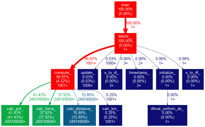
gprof2dot options
By default gprof2dot won’t display nodes and edges below a certain threshold.
Because our example has only a small number of subroutines/functions, we
have used the -n and -e options to set both thresholds to 0%.
Gprof2dot has several more options to, e.g. limit the depth of the tree, show only the descendants of a function or only the ancestors of another. Different coloring schemes are available as well.
$ gprof2dot --help
Usage:
	gprof2dot [options] [file] ...

Options:
  -h, --help            show this help message and exit
  -o FILE, --output=FILE
                        output filename [stdout]
  -n PERCENTAGE, --node-thres=PERCENTAGE
                        eliminate nodes below this threshold [default: 0.5]
  -e PERCENTAGE, --edge-thres=PERCENTAGE
                        eliminate edges below this threshold [default: 0.1]
  -f FORMAT, --format=FORMAT
                        profile format: axe, callgrind, hprof, json, oprofile,
                        perf, prof, pstats, sleepy, sysprof or xperf [default:
                        prof]
  --total=TOTALMETHOD   preferred method of calculating total time: callratios
                        or callstacks (currently affects only perf format)
                        [default: callratios]
  -c THEME, --colormap=THEME
                        color map: color, pink, gray, bw, or print [default:
                        color]
  -s, --strip           strip function parameters, template parameters, and
                        const modifiers from demangled C++ function names
  --colour-nodes-by-selftime
                        colour nodes by self time, rather than by total time
                        (sum of self and descendants)
  -w, --wrap            wrap function names
  --show-samples        show function samples
  -z ROOT, --root=ROOT  prune call graph to show only descendants of specified
                        root function
  -l LEAF, --leaf=LEAF  prune call graph to show only ancestors of specified
                        leaf function
  --depth=DEPTH         prune call graph to show only descendants or ancestors
                        until specified depth
  --skew=THEME_SKEW     skew the colorization curve.  Values < 1.0 give more
                        variety to lower percentages.  Values > 1.0 give less
                        variety to lower percentages
  -p FILTER_PATHS, --path=FILTER_PATHS
                        Filter all modules not in a specified path
Key Points
Don’t start to parallelize or optimize your code without having used a profiler first.
A programmer can easily spend many hours of work “optimizing” a part of the code which eventually speeds up the program by only a minuscule amount.
When viewing the profiler report, look for areas where the largest amounts of CPU time are spent, working your way down.
Pay special attention to areas that you didn’t expect to be slow.
In some cases one can achieve a 10x (or more) speedup by understanding the intrinsics of the language of choice.
Thinking in Parallel
Overview
Teaching: 30 min
Exercises: 15 minQuestions
How do I re-think my algorithm in parallel?
Objectives
Take the MD algorithm from the profiling example and think about how this could be implemented in parallel.
Our Goals
- Run as much as possible in parallel.
- Keep all CPU-cores busy at all times.
- Avoid processes/threads having to wait long for data.
What does that mean in terms of our MD algorithm?
Serial Algorithm
The Serial MD algorithm written as pseudo-code looks somewhat like this:
Pseudo Code
initialize()
step = 0

while step < numSteps:

  for ( i = 1;  i <= nParticles; i++ ):
    for ( j = 1;  j <= nParticles; j++ ):
      if ( i != j ) :
        calculate_distance(i, j)
        calculate_potential_energy(i, j)
        # Attributing half of the total potential energy of this pair to particle J.

        calculate_force(i, j)
        # Add particle J's contribution to the force on particle I.

  calculate_kinetic_energy()
  update_velocities()
  update_coordinates()

finalize()
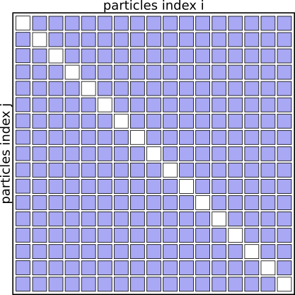
The algorithm basically works through a full matrix of size $N_{particles}^2$, evaluating the distances, potential energies and forces for all pairs (i,j) except for (i==j).
Graphically it looks like this:
Interaction Matrix: pair interactions (i!=j)
Optimized Serial Algorithm
We don’t need to evaluate the pairs of particles twice for (i,j) and (j,i), as the contribution to the potential energy for both is always the same, as is the magnitude of the force for this interaction, just the direction will always point towards the other particle.
We can basically speed up the algorithm by a factor of 2 just by eliminating redundant pairs and only evaluating pairs (i<j)
Pseudo Code
initialize()
step = 0

while step < numSteps:

  for ( i = 1;  i <= nParticles; i++ ):
    for ( j = 1;  j <= nParticles; j++ ):
      if ( i < j ):
        calculate_distance(i, j)
        calculate_potential_energy(i, j)
        # Attributing the full potential energy of this pair to particle J.

        calculate_force(i, j)
        # Add the force if pair (I,J) to both particles.

  calculate_kinetic_energy()
  update_velocities()
  update_coordinates()

finalize()
Interaction Matrix: pair interactions (i<j)
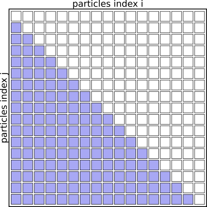
We don’t need to check for i<j at each iteration. The faster loop:
Pseudo Code
...
  for ( i = 1;  i <= nParticles; i++ ):
    for ( j = i + 1;  j <= nParticles; j++ ):
...
Simplistic parallelization of the outer FOR loop
A simplistic parallelization scheme would be to turn the outer for-loop (over index i) into a parallel loop. How this can be done will be covered on days two and three of the workshop.
The work could be distributed by assigning i=1,2 to CPU 1, i=3,4 to
CPU 2, and so on.
Pseudo Code
initialize()
step = 0

while step < numSteps:

  # Run this Loop in Parallel:
  for ( i = 1;  i <= nParticles; i++ ):

    for ( j = 1;  j <= nParticles; j++ ):
      if ( i < j ):
        calculate_distance(i, j)
        calculate_potential_energy(i, j)
        # Attributing the full potential energy of this pair to particle J.

        calculate_force(i, j)
        # Add the force if pair (I,J) to both particles.
  gather_forces_and_potential_energies()

  # Continue in Serial:
  calculate_kinetic_energy()
  update_velocities()
  update_coordinates()
  communicate_new_coordinates_and_velocities()

finalize()
Interaction Matrix: with simplistic parallelization
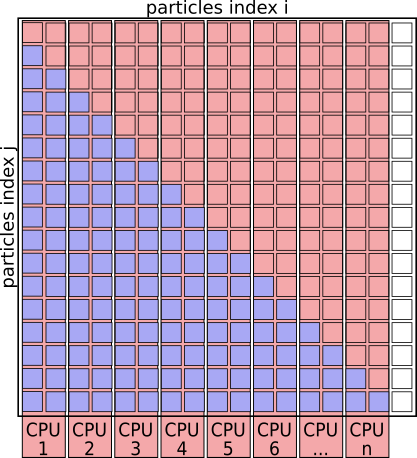
With this parallelization scheme CPU cores are idle ~50% of the time.
With this scheme CPU 1 will be responsible for many more interactions as CPU 8. This can easily improved by creating a pair-list upfront and evenly distributing particle-pairs for evaluation across the CPUs.
Pseudo Code: Using pair-list
initialize()
step = 0

while step < numSteps:

  # generate pair-list
  pair_list = []
  for ( i = 1;  i <= nParticles; i++ ):
    for ( j = 1;  j <= nParticles; j++ ):
      if ( i < j ):
        pair_list.append( (i,j) )

  # Run this Loop in Parallel:
  for (i, j) in pair_list:
    calculate_distance(i, j)
    calculate_potential_energy(i, j)
    # Attributing the full potential energy of this pair to particle J.

    calculate_force(i, j)
    # Add the force if pair (I,J) to both particles.
  gather_forces_and_potential_energies()

  # Continue in Serial:
  calculate_kinetic_energy()
  update_velocities()
  update_coordinates()
  communicate_new_coordinates_and_velocities()

finalize()
Using cut-offs
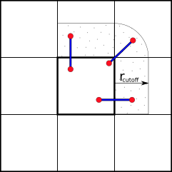
Still, this MD algorithm scales with $N_{particles}^2$, beyond which all forces and potential-energy contributions are truncated and treated as zero, can restore near-linear scaling. One way to do this is to bail out of the loop over the pair-list after computing the distance if it is larger than $r_{cut-off}$.
Further optimizations can be made by avoiding to compute the distances for all pairs at every step - essentially by keeping neighbor lists and using the fact that particles travel only small distances during a certain number of steps, however, those are beyond the scope of this lesson and are well described in text-books, journal publications and technical manuals.
Spatial- (or Domain-) Decomposition
When simulating large numbers of particles (~ 105)) and across many nodes, communicating the updated coordinates, forces, etc. every timestep can become a bottle-neck when using this Force- (or Particle-) Decomposition scheme, where particles are assigned to fixed processors as above.
To reduce the amount of communication between processors and nodes, we can partition the simulation box along its axes into smaller domains. The particles are then assigned to the processors depending on in which domain they are currently located. This way many pair-interactions will be local within the same domain and therefore handled by the same processor. For pairs of particles that are not located in the same domain, we can use e.g. the “eighth shell” method in which a processor handles those pairs, in which the second particle is located only in the positive direction of the dimensions, as illustrated below.
Domain Decomposition using Eight-Shell method
In this way, each domain only needs to communicate with neighboring domains in one direction as long as none of the domain’s dimension shorter than the longest cut-off.
Domain Decomposition not only applies to Molecular Dynamics (MD) but also to Computational Fluid Dynamics (CFD), Finite Elements methods, Climate- & Weather simulations and many more.
MD Literature:
- Larsson P, Hess B, Lindahl E.;
Algorithm improvements for molecular dynamics simulations.
Wiley Interdisciplinary Reviews: Computational Molecular Science 2011; 1: 93–108. doi:10.1002/wcms.3 - Allen MP, Tildesley DJ; Computer Simulation of Liquids. Second Edition. Oxford University Press; 2017.
- Frenkel D, Smit B; Understanding Molecular Simulation: From Algorithms to Applications. 2nd Edition. Academic Press; 2001.
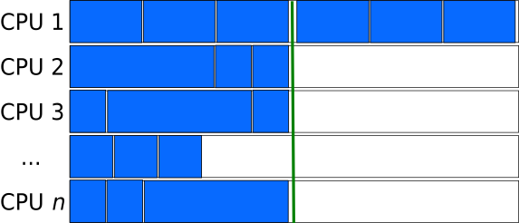
Load Distribution
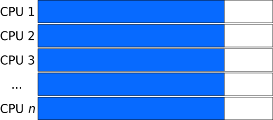
Generally speaking, the goal is to distribute the work across the available resources (processors) as evenly as possible, as this will result in the shortest amount of time and avoids some resources being left unused.
Ideal Load: all tasks have the same size
An ideal load distribution might look like this:
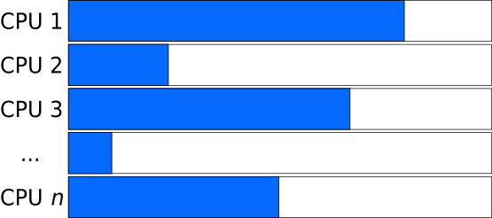
Unbalanced Load: the size of tasks differs
Whereas if the tasks that are distributed have varying length, the program needs to wait for the slowest task to finish. Such situations are even worse in cases where parallel execution is followed by a synchronization step, before proceeding to the next iteration of a larger-scope loop (e.g. next time-step, generation).
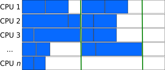
Balanced Load: pairing long and short tasks
In cases where the length of independent tasks can reasonably well be estimated, tasks of different lengths can be combined to “chunks” of similar length.
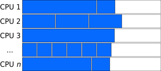
Larger Chunk-size evens out the size of tasks
Chunks consisting of many tasks (large chunk-size) can result relatively consistent lengths of the chunks, even if the lengths of the tasks are not pre-determined and have large variations. However, this can lead to situations, where a large fraction of the processors is left unused, when by chance, a chunk consists of many very long tasks, or as in the figure below, the number of chunks is sightly larger than the closest multiple of the processors.
Smaller Chunk-size can sometimes behave better
Smaller chunk-sizes (and therefore more chunks) are better in avoiding waste of resources during the last step, however are inferior in averaging out the different lengths of tasks.
Task-queues
Creating a queue (list) of independent tasks which are processed asynchronously can improve the utilization of resources especially if the tasks are sorted from the longest to the shortest.
However, special care needs to be taken to avoid race-conditions, where two processes take the same task from the stack. Having a dedicated manager- process to assign the work to the compute processes introduces overhead and can become a bottle-neck when a very large number of computing processes are involved.
This also increases the amount of communication needed.
Key Points
Efficiently parallelizing a serial code needs some careful planning and comes with an overhead.
Shorter independent tasks need more overall communication.
Longer tasks can cause other resources to be left unused.
Large variations of tasks-lengths can cause resources to be left unused, especially if the length of a task cannot be approximated upfront.
There are many textbooks and publications that describe different parallel algorithms. Try finding existing solutions for similar problems.
Domain Decomposition can be used in many cases to reduce communication by processing short-range interactions locally.